Check the data first
When a fit looks wrong, the circuit is an obvious suspect. But the measured data can be the problem. A Lin-KK test checks consistency between the real and imaginary parts of an EIS spectrum before equivalent-circuit fitting begins.
A researcher recently asked for help in our community. They had built an equivalent circuit from a published paper, yet the low-frequency end of the Nyquist plot would not fit. Repeated parameter adjustments made no difference.
Anyone who works with electrochemical impedance spectroscopy has probably seen this. The usual response is to add an element, change the diffusion model, and try again. This case points to a different question: is the dataset worth fitting in the first place?
1. Is the Warburg element really the problem?
The researcher used R0-p(CPE1,R1)-p(CPE2,R2)-W1. The two arcs at high and intermediate frequencies fit reasonably well. At low frequency, however, the measured points bend back toward the real axis. That shape does not match the 45° line of a semi-infinite Warburg element.
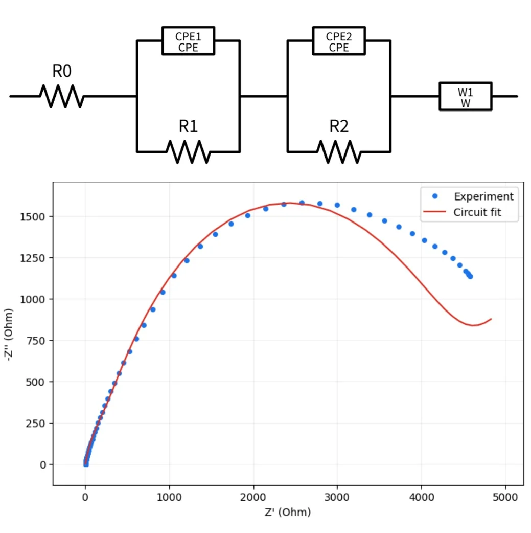
First check: the diffusion model
The first possibility was a poor choice of diffusion element. Three common Warburg elements have distinct low-frequency behavior:
Semi-infinite Warburg (W)
The low-frequency response remains close to a 45° line and extends indefinitely to the upper right.
Finite-length, transmissive boundary (Ws)
The low-frequency end gradually returns to the real axis. Its expression contains tanh.
Finite-length, blocking boundary (Wo)
The low-frequency end becomes an almost vertical capacitive tail. Its expression contains coth.
The measured return toward the real axis looks more like Ws. Another possibility was a third unresolved relaxation process rather than diffusion, which can be tested with R0-p(CPE1,R1)-p(CPE2,R2)-p(CPE3,R3).
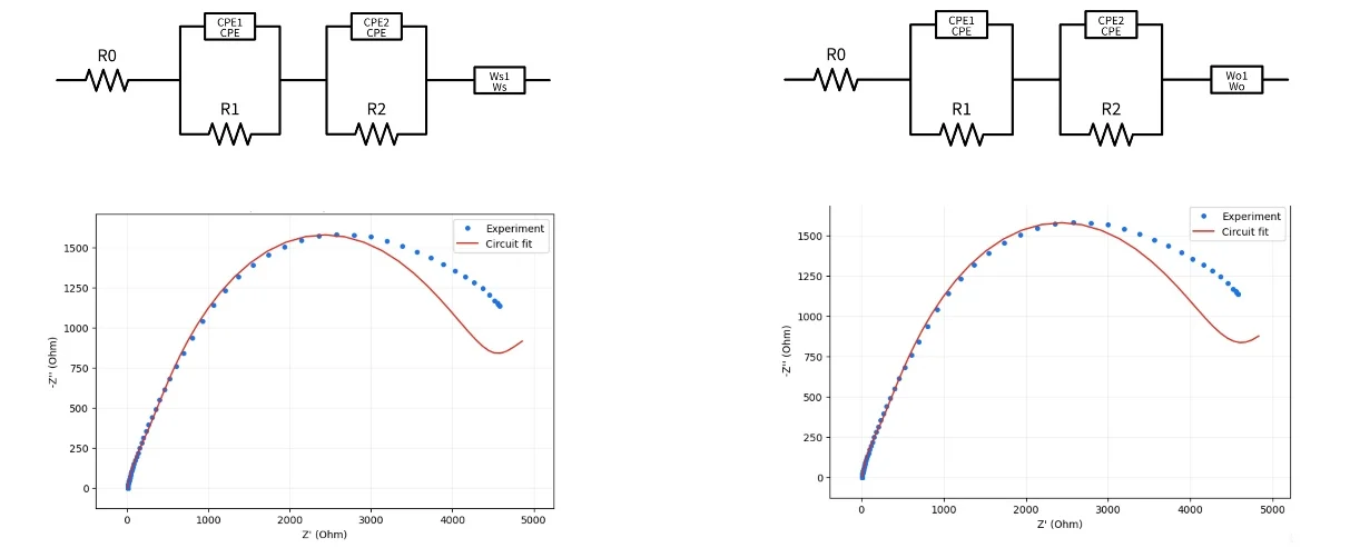
Neither change solved the problem. Replacing the diffusion element and adding another CPE-resistor pair both left a structured low-frequency residual. At that point, the model was no longer the only plausible cause.
2. Kramers-Kronig relations as a validity check
Equivalent-circuit analysis starts from three assumptions about the measured system:
Linearity
The perturbation is small enough that the response is proportional to the excitation.
Stability
The system does not drift, corrode, or undergo a side reaction during the test, and it can return to its initial state afterward.
Causality
The impedance response comes from the applied electrical perturbation rather than an independent spontaneous process.
When all three conditions hold, the real and imaginary parts of the impedance obey the Kramers-Kronig relations. If an EIS dataset fails this consistency test, it does not satisfy the basic assumptions of EIS. A more elaborate circuit may improve the numerical fit, but its fitted parameters have no physical meaning.
Lin-KK: a practical implementation
Direct K-K integration over a finite measured frequency range is awkward in practice. Oparic therefore uses the established Lin-KK method1-3. It fits the spectrum with a series of linear RC elements and quantifies departures from K-K consistency through the residuals.
Oparic fits Z', the real component, and uses the |Z|-normalized relative residual of Z'' as the main screening metric. For this case, the low-frequency problem is clear in the residual plot.
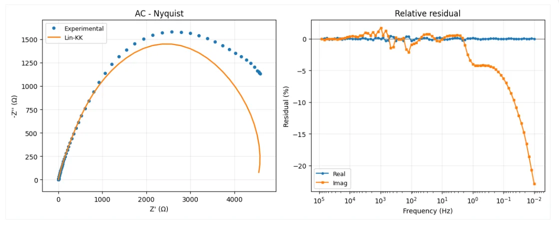
Above the 1% engineering threshold for imaginary RMSE
Above the 5% engineering threshold for a single point
The main departure is in the imaginary component at low frequency
Result: the dataset has poor K-K consistency, so the physical credibility of the equivalent-circuit fit is low. This is why changing diffusion elements and adding time constants did not fix the fit. The data are already distorted, and a more elaborate model cannot repair them.
3. What should you do with a K-K result?
Lin-KK is not meant to pass or fail a dataset with one number. It helps decide what to investigate next. Oparic reports one of three outcomes based on two engineering thresholds and the state of the fitted model:
| Outcome | Condition | Next step |
|---|---|---|
| Low residual | RMSE(Z'') ≤ 1% and maximum single-point imaginary residual ≤ 5% | Review the residual plot and experiment log before proceeding to equivalent-circuit fitting or DRT. |
| Review needed | Either imaginary-residual metric exceeds its engineering threshold | Look for frequency-dependent bias, low-frequency drift, outliers, and unstable test conditions. |
| Inconclusive | Too few valid points, failure to converge, the RC limit was reached, or a numerical error occurred | Check the data format, valid-point count, and frequency range. Do not interpret the result as material behavior. |
These are Oparic engineering screening thresholds, not acceptance criteria prescribed by the literature. The frequency pattern still matters: a sound residual should fluctuate randomly around zero rather than remain biased over part of the spectrum.
For this case, the 5.816% imaginary RMSE and 22.86% maximum single-point residual call for a repeat measurement before further analysis. Low-frequency points take a long time to collect and demand a stable system. A drifting electrode contact, an unsettled open-circuit potential, or a side reaction can distort a single run.
4. Common causes of poor low-frequency data
A large low-frequency imaginary residual is a common EIS problem. Four experimental issues deserve attention:
The system had not reached steady state
Starting EIS while the open-circuit potential is still drifting magnifies the effect during the long low-frequency measurement. Let the system settle first and check that OCP variation is within the millivolt range.
The electrode changed during the low-frequency scan
Corrosion, passive-film growth, dissolution, and other slow processes can change the electrode while the test is running. The final points no longer describe the same system as the first ones.
The perturbation amplitude was unsuitable
A large amplitude can produce a nonlinear response. A very small amplitude can leave the low-frequency signal with poor signal-to-noise ratio. Either problem weakens consistency.
Hardware or electrical contact was unstable
Poor electrode-clip contact, an unstable liquid-junction potential, or mains interference in the cables can all appear as low-frequency residuals.
5. Why Oparic includes K-K testing
During our first discussion of this case, we said that the next release would add K-K testing for an initial data-quality check. That feature is now available and can screen multiple spectra in one run.
Oparic / Quality report
EIS K-K consistency report
1 sample analyzed: 0 low residual, 1 review needed, 0 inconclusive.
- Method
- Lin-KK [1]
- Fit target
- Z'
- μ cutoff
- c = 0.85
- Maximum RC elements
- 50
- Low-frequency boundary
- Standard spectrum with an intercept
| Sample | Points | M | μ | RMSE(Z'') | RMSE(Z') | Max. imag. residual | Outcome |
|---|---|---|---|---|---|---|---|
| AC | 84 | 23 | 0.8455 | 5.816% | 0.1356% | 22.86% | Review needed |
How to read this result
Review needed: the imaginary relative residual exceeds an engineering threshold. Check for frequency-dependent bias, low-frequency drift, outliers, and unstable test conditions.
Researchers can spend hours adding elements, changing circuits, and tuning parameters without first asking whether the measured spectrum is fit for the task. K-K testing adds that check before circuit fitting:
If the data are consistent, move on to the circuit and mechanism.
If they are not, return to the experiment before forcing a clean-looking fit.
In Oparic, import the impedance data and run Lin-KK validation. The workflow calculates real and imaginary residuals, maximum single-point deviation, and model-stability metrics, then reports a screening result for each sample.
The point is to spend less time forcing circuits onto weak data and more time checking the experiment and interpreting the mechanism. If you have a difficult EIS fit or an idea for Oparic, join the discussion in our community.
References
- Schönleber, M., Klotz, D., and Ivers-Tiffée, E. (2014). A method for improving the robustness of linear Kramers-Kronig validity tests. Electrochimica Acta 131, 20-27. DOI: 10.1016/j.electacta.2014.01.034.
- Boukamp, B. A. (1995). A linear Kronig-Kramers transform test for immittance data validation. Journal of The Electrochemical Society 142, 1885-1894. DOI: 10.1149/1.2044210.
- Agarwal, P., Orazem, M. E., and Garcia-Rubio, L. H. (1992). Measurement models for electrochemical impedance spectroscopy: I. Demonstration of applicability. Journal of The Electrochemical Society 139, 1917-1927. DOI: 10.1149/1.2069522.