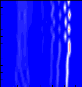
EIS/DRT Heatmap: Combining Multiple Samples' Relaxation Time Distributions into a 2D View

After running DRT analysis on a set of in-situ EIS measurements (across different potentials or time points) or a series of samples (different conditions, different concentrations), overlaying all the γ(τ) curves on a single line plot quickly becomes unreadable. This workflow combines them into a single τ-versus-sample heatmap, using color to visually convey how the intensity of a given relaxation process evolves across conditions.

Prerequisites

Choose one of two input types:

1. A drt_output/ directory produced by [EIS/DRT Analysis: Mapping Frequency-Domain Impedance to a Distribution of Relaxation Times](/docs/eis/drt) (a collection of samples with DRT already computed)
2. A directory of *_eis.csv files produced by [EIS Extraction: CHI Instruments Data Preprocessing](/docs/eis/extract_chi) or [In-Situ EIS Extraction: DH Instruments](/docs/eis/extract_in_situ_dh) (the program automatically runs DRT first, then plots)

At least 2 samples are required.

Procedure

Select a single directory. The program automatically:

1. Detects the directory layout (drt_output/ versus *_eis.csv)
2. Invokes the DRT solver if needed, caching each sample’s drt_data.csv to drt_heatmap/drt_output/<sample>/
3. Takes the intersection of all samples’ τ ranges, builds a 200-point logarithmic common grid, and linearly interpolates γ(τ) on the log-τ axis
4. Naturally sorts the sample names

Y-axis heuristic:

• If every sample name ends with an integer that can be extracted, and those integers are all distinct (e.g., in_situ_001, in_situ_002, …), the Y-axis mode is index. Those integers become the Y values, and the axis is labeled Sample Index.
• Otherwise the workflow falls back to ordinal mode: Y values are 1..N, and the Y-axis ticks use the sample names (attempted in Origin via LabTalk; on failure, the axis falls back to numeric ticks with a console warning).

The console prints the active mode for easy debugging.

Output

• drt_heatmap.png: matplotlib heatmap, with τ on the x-axis (log scale) and the y-axis determined by the heuristic
• drt_heatmap.opju: Origin project — the primary deliverable for subsequent editing. The x-axis stores log₁₀τ values (the title reads log₁₀τ); this avoids the visual mismatch you would get if you laid linearly-spaced matrix cells under a log axis
• drt_heatmap_clipped.png / drt_heatmap_clipped.opju: clipped heatmap variant. DRT results often contain a single dominant peak that is much higher than every other feature, which stretches the color scale and washes out all secondary relaxation processes. These two files cap the color-scale upper bound at 120% of the second-tallest peak height (computed with scipy.signal.find_peaks on each sample’s γ(τ); the program takes the largest “second peak” across all samples, then multiplies by 1.2). Cells above the threshold are rendered with the top color of the scale. Both variants are produced alongside the originals so you can compare them side-by-side. If every sample has only one peak, the clipped variant is skipped and a console message is printed.
• drt_heatmap_matrix.csv: the interpolated γ matrix (not clipped), with the first column holding sample names, the second column the Y values, and the remaining columns headed by τ
• samples_meta.json: records y_mode, y_label, input_kind, and the sample-to-Y-value mapping

In eis_csvs input mode, intermediate DRT results are also written to drt_heatmap/drt_output/<sample>/drt_data.csv for reuse.

Principle (Brief)

Each sample’s γ(τ) is interpolated onto a unified logarithmic τ grid, producing a matrix $\gamma_{i,j}$, where $i$ indexes the sample (y dimension) and $j$ indexes τ (x dimension). The heatmap encodes $\gamma_{i,j}$ as color, making the following readable at a glance:

• How the peak corresponding to a given relaxation process shifts along τ as conditions (potential/time) change
• Relative changes in peak intensity across samples

FAQ

• Why does it report “tau range no overlap”? If the frequency ranges of different samples do not overlap at all, the common τ grid cannot be constructed. Check the freq_hz column of the input data.
• How is the sample order determined? Natural sort: sample_001 < sample_002 < sample_010. If you do not want name-based ordering, rename the files beforehand.
• What if Origin custom Y ticks fail? The program catches the exception and falls back to numeric ticks. The .opju still opens correctly; only the Y-axis labels switch from sample names to 1, 2, 3, ....

Practical Tips

For in-situ EIS data (sampled by time or potential), embed strictly increasing integer indices in the sample names (e.g., _001, _002). The y-axis will then automatically use those indices as coordinates, making it easy to align with other in-situ curves.