EIS/Kramers–Kronig Consistency Validation
Use the Lin-KK algorithm to assess consistency between the real and imaginary components of EIS data before equivalent-circuit fitting or DRT analysis.
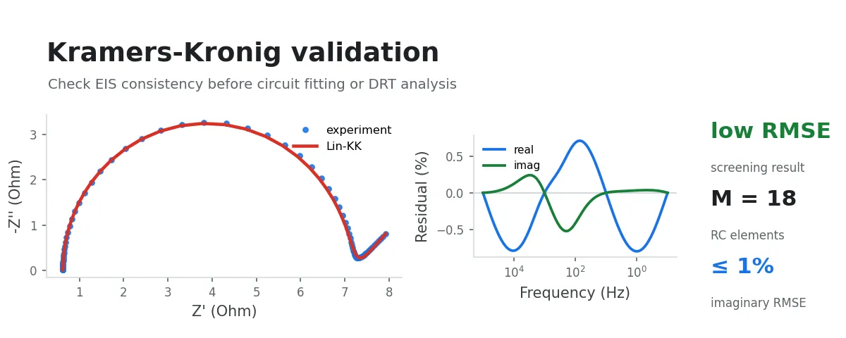
The Kramers–Kronig relations are used to assess consistency between the real and imaginary components of EIS data. Deviations may result from nonlinearity, nonstationarity, a finite frequency range, or measurement error, but this test alone cannot identify the specific cause.
KK validation is useful for assessing data quality before equivalent-circuit fitting, DRT analysis, or sample comparison. Its results do not select an equivalent circuit and are not sufficient to validate a material mechanism.
When to Use This Workflow
Consider running KK validation in the following situations:
- You are preparing to fit an equivalent circuit and want to assess data quality first
- A Nyquist or Bode plot contains a few suspicious frequency points, but it is unclear whether they should be removed
- The low-frequency region may be affected by drift, changes in sample state, or an excessively long measurement
- You need to compare samples from the same batch and want to identify clearly unstable datasets first
- Fitted parameters are unstable and you want to distinguish data-quality issues from model-selection issues
Before running this workflow, use EIS Plotting: Nyquist and Bode to inspect the original Nyquist and Bode curves.
Input Data
Select a folder containing instrument-exported EIS data, or multi-select several raw files. Common text, CSV, Excel, EC-Lab .mpr, Gamry .dta, and VersaStudio .par formats are supported.
You can also provide standardized EIS CSV files. Each file must contain at least:
| Column | Meaning |
|---|---|
freq_hz | Frequency |
z_real_ohm | Real component of impedance |
z_imag_ohm | Imaginary component of impedance |
Analysis Procedure
After you select the data, the interface displays the original Nyquist plots for all samples. You can hover to inspect frequency and impedance values, zoom, pan, and double-click to reset the view. The x- and y-axes use the same scale per data unit so the spectral shape is not distorted by axis scaling.
The workflow recommends a low-frequency boundary mode from the spectral shape at the lowest frequencies of each sample. It lists the minimum frequency, the starting and ending values of over the final low-frequency segment, and the corresponding recommendation. If all samples receive the same recommendation, the interface preselects that mode. If the recommendations differ, the interface asks you to process the samples in separate groups according to the table. The automatic recommendation only assists configuration; the final choice should be based on the original Nyquist and Bode spectra.
The workflow only reads the source data and writes all analysis results to a separate output directory.
Interpret the results using the report classification, the frequency distribution of the residuals, and the original impedance spectrum together. Do not rely on a single summary metric.
Method and Low-Frequency Boundary Setting
This workflow uses the Lin-KK algorithm [1]. It fits (the real component) and uses the -normalized relative residual of as the primary screening metric.
Two low-frequency boundary modes are available:
- Conventional spectrum with a low-frequency intercept: the lowest-frequency region has reached or is approaching the real-axis intercept; no series-capacitance term is added.
- No low-frequency intercept / low-frequency capacitive tail: the lowest-frequency region continues as a capacitive tail; a series-capacitance term is added.
The series-capacitance term increases the degrees of freedom of the auxiliary model, so the workflow does not select the low-frequency boundary model automatically from residual magnitude. Your selection is recorded in the boundary_mode and add_cap columns of kk_summary.csv.
Output
Results are saved in a kk_validation_output directory under the input directory.
Each successfully analyzed sample produces:
{sample}_kk_fit.csv: experimental impedance, Lin-KK fitted impedance, and relative residuals for the real and imaginary components.{sample}_kk_fit.png: Nyquist comparison and residual plots.
Batch-level files include:
kk_summary.csv: point count,M,mu,RMSE(Z''),RMSE(Z'), maximum imaginary-component residual, low-frequency boundary model, and conclusion for every sample.
After you select Confirm and generate, you can also export:
kk_validation.opju: an Origin project containing the Nyquist comparison and residual plots.
How to Interpret the Results
The report uses three conclusion levels:
| Conclusion | Meaning |
|---|---|
| Low residual | The relative residual of the imaginary component is below the engineering thresholds; this classification alone is not sufficient evidence that the data is valid |
| Review required | The relative residual of the imaginary component exceeds an engineering threshold; inspect the data for systematic, frequency-dependent deviation |
| Indeterminate | The current result is insufficient for classification, possibly because there are too few valid points, the frequency range is limited, or numerical values are abnormal |
The workflow uses the relative-residual RMSE(Z'') as the primary screening metric; the real-component residual is provided only as a reference. A result is classified as low residual when RMSE(Z'') ≤ 1% and the maximum single-point relative residual of the imaginary component is at most 5%. These thresholds are Oparic engineering criteria, not acceptance criteria prescribed by the literature. Whether the residuals fluctuate randomly around zero across frequency remains important when interpreting KK consistency.
Also inspect {sample}_kk_fit.png:
- In the Nyquist comparison, the Lin-KK fitted curve should broadly follow the experimental points.
- In the residual plot, residuals should ideally fluctuate randomly around zero rather than remain positive or negative over a frequency interval.
- A clear deviation at low frequency commonly indicates sample drift, an excessively long measurement, nonlinear response, or unstable low-frequency points.
- If only isolated frequency points deviate, review the original experiment records for contact disturbances, instrument range switching, or data-export anomalies.
Method Notes
The Lin-KK algorithm fits an impedance spectrum with a set of RC elements distributed over time constants, then compares the fitted and measured values [1]. See [2, 3] for the KK relations and [4] for EIS data-analysis methods.
High KK residuals may result from nonlinearity, nonstationarity, a finite frequency range, or measurement error. This validation cannot identify the source of a deviation by itself, nor can it prove that an equivalent circuit or reaction mechanism is correct.
Subsequent Analysis
- Low residual: review the residual plot and experiment records, then proceed to EIS Equivalent-Circuit Fitting or EIS/DRT Analysis.
- Review required: use EIS Plotting: Nyquist and Bode to inspect low-frequency drift, outliers, and measurement stability.
- Indeterminate: check the data format, frequency range, and number of valid points; do not interpret the current result directly as material behavior.
References
- Schönleber, M., Klotz, D., and Ivers-Tiffée, E. (2014). A method for improving the robustness of linear Kramers-Kronig validity tests. Electrochim. Acta 131, 20-27. https://doi.org/10.1016/j.electacta.2014.01.034.
- Boukamp, B.A. (1995). A linear Kronig-Kramers transform test for immittance data validation. J. Electrochem. Soc. 142, 1885-1894. https://doi.org/10.1149/1.2044210.
- Agarwal, P., Orazem, M.E., and Garcia-Rubio, L.H. (1992). Measurement models for electrochemical impedance spectroscopy. I. Demonstration of applicability. J. Electrochem. Soc. 139, 1917-1927. https://doi.org/10.1149/1.2069522.
- Orazem, M.E., and Tribollet, B. (2017). Electrochemical Impedance Spectroscopy, 2nd ed. (John Wiley & Sons). https://doi.org/10.1002/9781119363682.