EIS Equivalent-Circuit Fitting

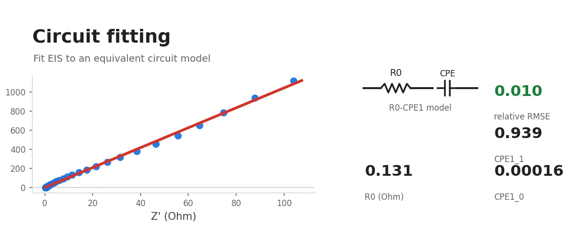
After reviewing the Nyquist and Bode plots, you may want to convert the resistance, capacitance, diffusion, or transmission-line features in the spectrum into comparable parameters. This workflow is designed for that step.

It fits EIS data with an equivalent circuit and outputs fitted curves, parameter tables, and residual diagnostics for each sample. It is useful for comparing samples, treatment conditions, or interfacial kinetic changes before and after cycling.

Input Data

Select a folder containing instrument-exported raw EIS data, or multi-select a group of raw EIS data files. Common text, CSV, Excel, EC-Lab .mpr, Gamry .dta, and VersaStudio .par files can be recognized automatically.

Procedure

Select EIS Data: choose a folder, or multi-select a group of files from the same experiment.
Select a Circuit Model: use one of the preset models, or type a custom circuit expression.
Configure Fit Parameters: use automatic initial values and recommended bounds by default; when needed, enter parameter rules for initial values, bounds, or fixed values.
Review the Fit: after fitting, inspect the Nyquist fit, frequency-dependent residuals, and KK checks before using the parameters in a report or manuscript.
Optionally Export a Word Analysis Report: generate an illustrated .docx batch report for archiving, communication, and further editing.
Optionally Export an Origin Project: generate an .opju file if you need further figure editing.

Circuit Expression Syntax

Use - for series connection, such as R0-C1.
Use p(...) for parallel connection. For example, R0-p(C1,R1) means a series resistance followed by a capacitor/resistor parallel branch.
Full-width parentheses, Chinese commas, Chinese dash-like connectors, and P(...) are accepted and normalized automatically. For example, R0－P（C1，R1）－W1 is treated as R0-p(C1,R1)-W1.
Use numeric suffixes to distinguish elements of the same type, such as R0, R1, and C1.
If an element is entered without a numeric suffix, the workflow adds one automatically. For example, R0-p(C1,R1)-G-L is treated as R0-p(C1,R1)-G1-L1.
If element identifiers are repeated, the workflow automatically assigns unique identifiers to later elements and shows both expressions. For example, R0-p(CPE1,R1)-p(CPE1,R1) is normalized to R0-p(CPE1,R1)-p(CPE2,R2). After you confirm the normalized model, parameter settings, fitting, and exports all use the confirmed expression.
Multi-parameter elements are expanded into multiple fit parameters. For example, CPE1 corresponds to CPE1_0 and CPE1_1; Wo1 corresponds to Wo1_0 and Wo1_1.

Common preset models:

R0-C1 — series resistance + a single capacitor
R0-p(C1,R1) — series resistance + parallel capacitor/resistor (the typical double-layer capacitance with charge-transfer resistance)
R0-CPE1 — series resistance + constant phase element (non-ideal capacitance)
R0-p(CPE1,R1) — series resistance + parallel CPE/resistor (useful for rough interfaces, porous structures, or distributed time constants)
R0-p(C1,R1)-W1 — series resistance + (parallel capacitor/resistor) + Warburg (adds semi-infinite diffusion impedance after interfacial charge transfer)

See the "Element Overview" section below for the full list of supported elements with their units and impedance equations.

How to Configure Fit Parameters

In most cases, use the default settings. All parameters participate in the fit, while the workflow estimates initial values separately for each sample and uses recommended parameter bounds.

The parameter section lists every parameter in the current circuit with its units and recommended range. Leave the rule input blank to fit every parameter with automatic initial values and recommended bounds. Enter rules only when you need to override those settings:

R0=1.0: fix R0 at 1.0, excluding it from optimization and fitted confidence intervals.
R1~100: fit R1 with an initial value of 100.
R1>0 or R1<=1e6: set a one-sided fitting bound.
0<CPE1_1<=1: set both lower and upper bounds.
R1~100, 0<R1<1e6: combine an initial value with bounds.

Separate rules with commas or semicolons. Full-width punctuation from Chinese input methods is also accepted. Parameters omitted from the rules retain automatic settings. Every rule applies to all samples selected for the run.

Fixed values should come from independent measurements, geometric relationships, or an explicit model hypothesis. A value obtained from one fit is not automatically a reliable physical prior. When a fixed value or input bound exceeds the recommended range, the workflow records and displays a warning but allows an expert user with a justified reason to continue. If an automatic initial value falls outside input bounds, it is moved inside those bounds and the adjustment is recorded.

If the initial values are uncertain but the circuit is relatively complex, you can enable global optimization. It explores a wider parameter space, but it also takes noticeably longer.

Output

Each sample produces:

*_circuit_fit.csv: experimental impedance, fitted impedance, and real/imaginary residuals.
*_circuit_fit.png: Nyquist comparison between experimental points and the circuit fit, with frequency-dependent relative residuals.
circuit_summary.json: circuit expression, original parameter rules, resolved initial values and bounds for each parameter, fixed values, warnings, fitted parameters, confidence intervals, and RMSE.

Batch-level results include:

fit_summary.csv: fitted parameters for all samples.
fit_diagnostics.csv: fit quality and simple diagnostic information.
fit_diagnostics.md: a quick-readable fitting report.
filter_circuit_report.docx: an illustrated analysis report generated after clicking Export Word report.
filter_circuit_fit.opju: optional Origin project.

The fitting report also contains a Markdown table with one row per sample and parameter. Its "Fixed rule" column uses the parameter=value format so that a result can be copied and fixed on a later run. In a batch run, a manually entered fixed value applies to every sample, so verify that the copied value is appropriate for the entire batch.

Word Analysis Report

The workflow exports one filter_circuit_report.docx for each fitting batch. The report includes:

sample names, source file names, detected formats, file sizes, modification times, valid point counts, and frequency ranges;
the preprocessing steps actually applied, plus explicit confirmation that smoothing, outlier removal, blank subtraction, and baseline correction were not applied;
the circuit expression, fitting method, Lin-KK settings, parameter rules, initial guesses, bounds, fixed parameters, and parameter warnings;
batch fitting summaries, data-integrity/high-frequency-real/KK checks, and necessary warnings;
the circuit diagram, per-sample Lin-KK figures, Nyquist fitting figures, and complete parameter tables;
interpretation limits, analysis workflow version, analysis time, and scientific package versions.

The report is generated from data available in the current fitting run. Lin-KK and fitting-quality labels are engineering screening aids only; they do not by themselves establish a unique circuit mechanism or parameter interpretation.

If the button shows Word export unavailable, upgrade Oparic and try again; fitting remains available.

How to Judge Whether the Fit Is Trustworthy

The fitted line should closely follow the experimental points in the Nyquist plot, especially near the semicircle apex, low-frequency diffusion tail, and high-frequency intercept.
A smaller rmse_rel means a smaller overall residual, but a small residual does not prove that the model is unique or mechanistically correct.
Parameters should have reasonable magnitudes. For example, solution resistance should be positive, and the CPE exponent is usually between 0 and 1.
Do not interpret a single parameter in isolation. Compare the circuit structure, fitted plot, residuals, and electrochemical context together.
If several circuits fit well, prefer the simpler model with clearer physical meaning.

Element Overview

The following table lists the equivalent-circuit elements supported by this workflow. Let $\omega = 2\pi f$ and $j=\sqrt{-1}$ .

Element	Fit Parameters	Units	Common Meaning
`R`	`R0`	$\Omega$	Ohmic, solution, or charge-transfer resistance
`C`	`C0`	$\mathrm{F}$	Ideal capacitance, such as ideal double-layer capacitance
`L`	`L0`	$\mathrm{H}$	Inductance or high-frequency parasitic response
`W`	`W0`	$\Omega\,\mathrm{s}^{-1/2}$	Semi-infinite Warburg diffusion impedance
`Wo`	`Wo0_0`, `Wo0_1`	$\Omega$ , $\mathrm{s}$	Open finite-space Warburg element
`Ws`	`Ws0_0`, `Ws0_1`	$\Omega$ , $\mathrm{s}$	Short finite-length Warburg element
`CPE`	`CPE0_0`, `CPE0_1`	$\Omega^{-1}\,\mathrm{s}^{\alpha}$ , dimensionless	Constant phase element for non-ideal capacitance
`La`	`La0_0`, `La0_1`	$\mathrm{H}\,\mathrm{s}$ , dimensionless	Modified inductance for non-ideal inductive behavior
`G`	`G0_0`, `G0_1`	$\Omega$ , $\mathrm{s}$	Gerischer element for coupled reaction-diffusion response
`Gs`	`Gs0_0`, `Gs0_1`, `Gs0_2`	$\Omega$ , $\mathrm{s}$ , dimensionless	Finite-length Gerischer element
`K`	`K0_0`, `K0_1`	$\Omega$ , $\mathrm{s}$	Single RC relaxation process
`Zarc`	`Zarc0_0`, `Zarc0_1`, `Zarc0_2`	$\Omega$ , $\mathrm{s}$ , dimensionless	Depressed semicircle or Cole-Cole-type relaxation
`TLMQ`	`TLMQ0_0`, `TLMQ0_1`, `TLMQ0_2`	$\Omega$ , $\mathrm{F}\,\mathrm{s}^{\gamma-1}$ , dimensionless	Simplified transmission-line model with non-ideal interfacial capacitance
`T`	`T0_0`, `T0_1`, `T0_2`, `T0_3`	$\Omega\,\mathrm{m}^2$ , $\Omega\,\mathrm{m}^2$ , dimensionless, $\mathrm{s}$	Macrohomogeneous porous-electrode transmission-line model

Appendix: Element Equations

The series and parallel combination rules are:

$Z_{\mathrm{series}} = Z_1 + Z_2 + \cdots + Z_n$

$Z_{\mathrm{parallel}} = \frac{1}{\frac{1}{Z_1}+\frac{1}{Z_2}+\cdots+\frac{1}{Z_n}}$

The impedance expressions for the supported elements are:

Element	Equation
`R`	$Z_R=R$
`C`	$Z_C=\frac{1}{j\omega C}$
`L`	$Z_L=j\omega L$
`W`	$Z_W=\frac{A_W(1-j)}{\sqrt{\omega}}$
`Wo`	$Z_{Wo}=\frac{Z_0}{\sqrt{j\omega\tau}}\coth(\sqrt{j\omega\tau})$
`Ws`	$Z_{Ws}=\frac{Z_0\tanh(\sqrt{j\omega\tau})}{\sqrt{j\omega\tau}}$
`CPE`	$Z_{CPE}=\frac{1}{Q(j\omega)^\alpha}$
`La`	$Z_{La}=L(j\omega)^\alpha$
`G`	$Z_G=\frac{R_G}{\sqrt{1+j\omega t_G}}$
`Gs`	$Z_{Gs}=\frac{R_G}{\sqrt{1+j\omega t_G}\tanh(\phi\sqrt{1+j\omega t_G})}$
`K`	$Z_K=\frac{R}{1+j\omega\tau_k}$
`Zarc`	$Z_{arc}=\frac{R}{1+(j\omega\tau_k)^\gamma}$
`TLMQ`	$Z_{TLMQ}=\sqrt{R_{ion}Z_S}\coth\sqrt{\frac{R_{ion}}{Z_S}}$ , where $Z_S=\frac{1}{Q_S(j\omega)^\gamma}$
`T`	$Z_T=A\frac{\coth\beta}{\beta}+B\frac{1}{\beta\sinh\beta}$ , where $\beta=(a+j\omega b)^{1/2}$

For multi-parameter elements, _0, _1, _2, and _3 follow the parameter order in the equation. For example, CPE1_0 is $Q$ and CPE1_1 is $\alpha$ ; Wo1_0 is $Z_0$ and Wo1_1 is $\tau$ ; Gs1_0, Gs1_1, and Gs1_2 are $R_G$ , $t_G$ , and $\phi$ , respectively. Use the units listed in the Element Overview table above.

Practical Tips

If you have not yet inspected the raw EIS curves, use EIS Plotting: Nyquist and Bode first to review the Nyquist and Bode plots. If the curve contains obvious outliers, inductive tails, or low-frequency drift, address the data quality before fitting an equivalent circuit.

If the circuit parameters are unstable or difficult to interpret, use EIS/DRT Analysis to inspect the distribution of relaxation times, then return to this workflow with a more physically motivated circuit structure.